A surface, a tangent plane, a normal line
I set out to plot a simple 3d surface \( z=x^2+y^2\), together with its
tangent plane and a normal line at the point \( (1,1,2) \).
I knew that it was easy to plot two curves on the same axes
using the plot2d functionality in Maxima.
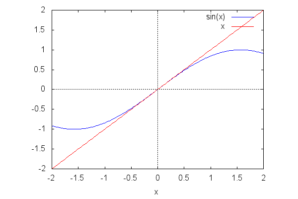
Here it is using wxplot2d
(note that plot2d with the same calling sequence as below
draws the plot in a new window rather inline, more on that later...)
| (%i1) | wxplot2d([sin(x),x],[x,-2,2]); |
 \[\mathrm{\tt (\%o1) }\quad \]
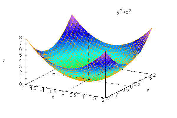
So here's the surface alone using wxplot3d. Notice the calling sequence for a single surface is completely analogous to wxplot2d, and the labels, legend and color are pretty nice by default:
| (%i2) | wxplot3d(x^2+y^2, [x,-2,2],[y,-2,2]); |
 \[\mathrm{\tt (\%o2) }\quad \]
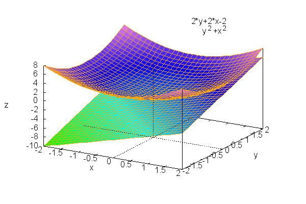
To draw two surfaces in the same plot using wxplot3d, notice the slightly different way we need to use the square brackets...they enclose both surfaces and the specification of the x and y ranges.
| (%i5) | wxplot3d([x^2+y^2, 2*x+2*y-2,[x,-2,2],[y,-2,2]]); |
 \[\mathrm{\tt (\%o5) }\quad \]
So far, so good. I couldn't figure out how to draw the normal line on the same plot using wxplot3d. I have done something similar with wxdraw3d, so here's a step by step, with a few fumbles and recoveries along the way. First the bare bones:
| --> |
wxdraw3d(explicit(x^2+y^2,x,-2,2,y,-2,2), explicit( 2*x+2*y-2,x,-2,2,y,-2,2))$ |
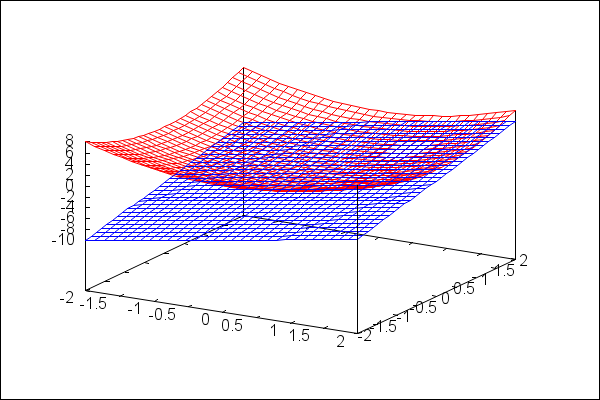
Kinda drab, no? We can control the colors in lots of ways. Here we set the color independently for each surface. Notice the modifiers go before the specification of the surface.
| (%i29) |
wxdraw3d( color=red, explicit(x^2+y^2,x,-2,2,y,-2,2), color=blue, explicit( 2*x+2*y-2,x,-2,2,y,-2,2))$ |
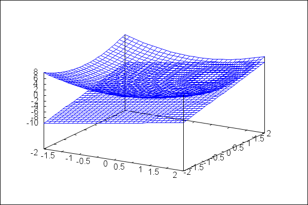
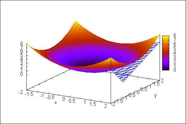
We can also get the cool multicolored effect with enhanced3d=true. Notice the axes don't get labels automatically with wxdraw3d. I add them here. And another cool thing: notice we can specify the plane implicitly in the standard form we learned in multivariable calculus:
| --> |
wxdraw3d(enhanced3d=true, xlabel="x",ylabel="y", explicit(x^2+y^2,x,-2,2,y,-2,2), enhanced3d=false,color=blue, implicit( z-2=2*(x-1)+2*(y-1),x,-2,2,y,-2,2,z,0,8)); |
 \[\mathrm{\tt (\%o36) }\quad \]
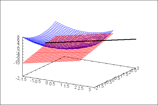
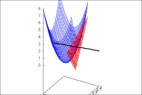
Now for the normal line. This part really is cool, but beware: Without some alteration, the plot is entirely unusable for showing the normal line:
| --> |
wxdraw3d(color=blue, explicit(x^2+y^2,x,-2,2,y,-2,2), color=red, implicit( z-2=2*(x-1)+2*(y-1),x,-2,2,y,-2,2,z,0,8), color=black,line_width=3, parametric(2*t+1,2*t+1,-t+2,t,-1,1)); |
 \[\mathrm{\tt (\%o37) }\quad \]
Seriously, I checked my line a dozen times, thinking that I had
the formula wrong because the picture doesn't get the normal line
perpendicular to the surface. Not.At.All.
I looked around on the web, and thanks to the Maxima community,
I learned how to make the squished-up scale on the vertical
axis proportional to the horizontal scales, and that fixed the line:
| (%i41) |
wxdraw3d(color=blue, explicit(x^2+y^2,x,-2,2,y,-2,2), color=red, implicit( z-2=2*(x-1)+2*(y-1),x,-2,2,y,-2,2,z,0,8), color=black,line_width=3, parametric(2*t+1,2*t+1,-t+2,t,-1,1), proportional_axes=xyz); |
 \[\mathrm{\tt (\%o41) }\quad \]
At last. Maybe a few changes in the colors would be nicer.
Maybe surface_hide=true.
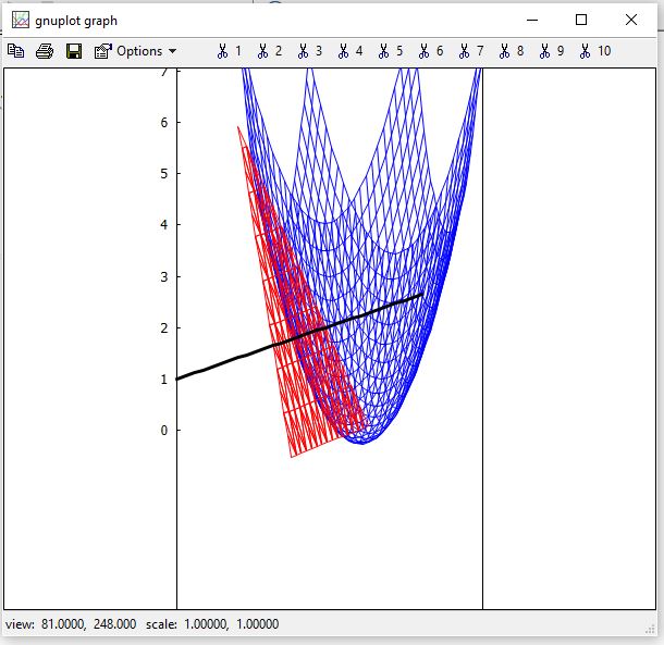
But what I really wanted to do is click my mouse on that drawing and rotate it!
Turns out that the draw3d (rather than wxdraw3d) with the same calling sequence
opens the 3d plot in a new window that has the usual mouse-click-drag rotation
we've all come to expect from other graphics programs. Here's the command,
followed by a screenshot of the rotated surface-plane-line complex.
| (%i42) |
draw3d(color=blue, explicit(x^2+y^2,x,-2,2,y,-2,2), color=red, implicit( z-2=2*(x-1)+2*(y-1),x,-2,2,y,-2,2,z,0,8), color=black,line_width=3, parametric(2*t+1,2*t+1,-t+2,t,-1,1), proportional_axes=xyz); |
Figure 1: C:\Users\Rick\Documents\draw3dplot.JPG