For the initial value problem \[ \ddot{x}+2\dot{x}+2x = 2\cos(3t), x(0)=1, \dot{x}(0)=0 \] Find the stead-state solution and estimate a time \( t \) beyond which the absolute value of the transient solution remains less than 1/100.
| (%i20) | eq: 'diff(x,t,2)+2*'diff(x,t)+2*x = 2*cos(3*t); |
| (%i21) | gsol: ode2(eq,x,t); |
| (%i23) | psol: ic2(gsol,t=0,x=1,'diff(x,t)=0); |
| (%i25) | wxplot2d(rhs(psol),[t,0,10]); |
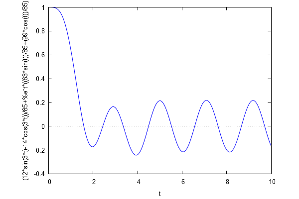 \[\mathrm{\tt (\%o25) }\quad \]
| (%i26) | eqH: 'diff(x,t,2)+2*'diff(x,t)+2*x = 0; |
| (%i27) | gsolH: ode2(eqH,x,t); |
Here's the specific solution: the general solution of the nonhomogeneous equation minus the general solution of the associated homogeneous equation
| (%i35) | ssol: rhs(gsol)-rhs(gsolH); |
And so here's the transient solution...the particular solution minus the specific solution
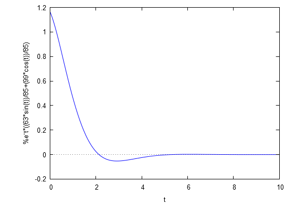
| (%i36) | tsol: rhs(psol)-ssol; |
| (%i37) | wxplot2d(tsol,[t,0,10]); |
 \[\mathrm{\tt (\%o37) }\quad \]
Now let's hunt and peck for t beyond which the transient solution is less than 0.01 to see that this value of t is something between 4 and 5...certainly t=5 is safe.
| (%i49) | block( ev(tsol,t=3),float(%%)); |
| (%i50) | block( ev(tsol,t=4),float(%%)); |
| (%i51) | block( ev(tsol,t=5),float(%%)); |
| (%i52) | tsol; |
On the other hand, we could make an estimate using the sinusoidal oscillator formula and the fact that \( |\cos(u)| \le 1 \)
| (%i66) | block(sqrt( (63/85)^2 + (99/85)^2 ),float(%%)); |
| (%i67) | 0.01/%; |
| (%i68) | -log(%); |
And finally, we could just use the built-in numerical rootfinder:
| (%i78) | find_root(abs(tsol)-0.01,t,4,5); |